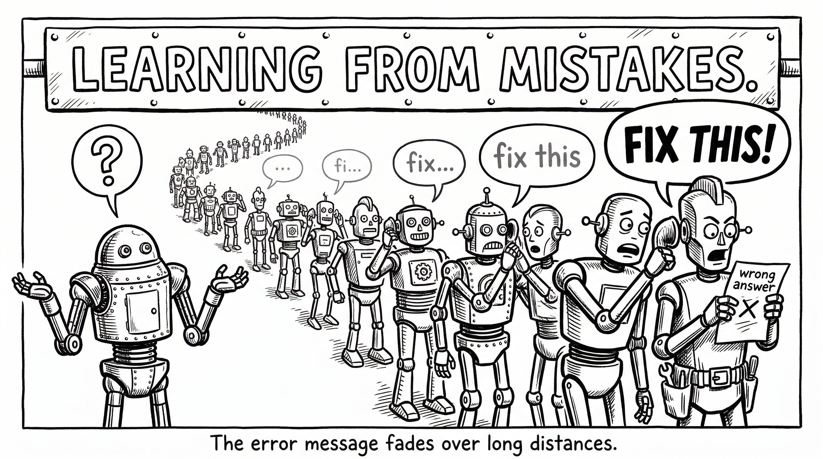
You’ll learn how Backpropagation Through Time (BPTT) unrolls an RNN so gradients can flow backward from the loss to every shared weight. You’ll also see why repeated multiplication creates vanishing or exploding gradients, and how gradient clipping keeps training stable.
For your first pass, follow the backward-pass animation and the six-step explanation. The detailed derivative and implementation sections are optional. In the GPT training lab, you’ll use automatic differentiation while keeping this same idea: trace the loss back to the weights that produced it.
In the forward pass, we computed predictions and measured our error. The backward pass calculates how a change to each weight affects that error. We use those gradients to choose an update.
Why Gradients Matter
How do we know which direction to adjust each weight? Explore below. Drag the weight along the loss curve and watch what happens when you nudge it:
What Is a Gradient?
Drag on the curve to move the weight
Model:prediction = w × 2, target = 6, Loss = (prediction − 6)²
Weight5.50
Loss25.00
Gradient+20.00
Sensitivityhigh
w − ε = 5.15→Loss = 18.49
w + ε = 5.85→Loss = 32.49
Gradient ≈ (32.49 − 18.49) / 0.70 = 20.00
← Positive gradient: loss increases when w increases, so decrease w to reduce loss.
What to look for:
Drag the dot along the curve. Far from the minimum, the loss is high and the gradient is large (steep slope). Near the minimum, everything flattens out.
The nudge (the two smaller dots) shows the loss at w+ε and w−ε. The ratio of loss change to weight change IS the gradient.
The sign tells direction: a positive gradient means “loss goes up when w goes up,” so we decrease w. A negative gradient means the opposite.
The magnitude tells sensitivity: a large gradient means this weight has a big effect on the error right now. A small gradient means we’re close to where we want to be.
Click Gradient Step to apply one update, or Train to watch gradient descent converge step by step.
A gradient tells us: “If I nudge this weight by a tiny amount, how much does the loss change?” Training is just repeated gradient descent: at each step, adjust every weight in the direction that reduces the error.
See the Backward Pass First
Before diving into the mechanics, explore the backward pass interactively. Click any node to inspect its gradient — watch how the error signal flows backward from the loss through every computation:
RNN Computation Graph
Forward
vectorsmatricesopsactivations
100%
V=0H=4L=—
What to look for:
Gradients start at the loss (right side) and flow leftward through time
Each hidden state receives gradients from two sources: its own output and the next timestep
The gradient signal gets weaker as it travels further back in time — this is the vanishing gradient problem in action
The Challenge: Shared Weights
In a feedforward network, each layer has independent weights. In an RNN, the same weights are reused at every timestep:
Feedforward: x → W₁ → W₂ → W₃ → y (3 separate weight matrices)RNN: x₀ → W → h₁ → W → h₂ → W → h₃ (same W reused)
Consequence: we must account for all uses of the weight across time — the total gradient sums contributions from every timestep. This is what makes RNN backpropagation special — and why it’s called Backpropagation Through Time (BPTT).
The Chain Rule: Our Main Tool
The backward pass is built entirely on the chain rule. Think of it as a chain of gears — pushing one gear moves the next, which moves the next. The total effect is the product of each link.
Everyday analogy: If you eat 2x more food → you gain 3x more weight → your doctor is 1.5x more concerned. The total effect of eating on doctor-concern is 2 x 3 x 1.5 = 9x. That’s the chain rule.
In our network, the loss depends on the output, which depends on the hidden state, which depends on the weights. We compute these pieces one at a time, starting from the loss and working backward — hence “backward pass.”
The Six Steps (Intuition)
Here’s what happens at each step of the backward pass, without the math:
Step
What happens
Intuition
1. Output error
Compare prediction to target
”How far off was I?” — subtract the correct answer
2. Output weights
Use error to update output layer
”How should I adjust my scoring?“
3. Hidden gradient
Error flows into the memory
Gets error from two sources: current output + future timesteps
4. Through tanh
Error passes through squashing
Saturated neurons (near ±1) block the gradient — only 2% passes through
5. Hidden weights
Accumulate weight updates
Same weights used everywhere, so add up contributions from all timesteps
6. Time chain
Send error one step further back
This is the “through time” — the loop that repeats for every timestep
Key insight about Step 4: When the hidden state is saturated (near +1 or -1), the gradient gets nearly killed. This is one reason RNNs struggle with long sequences — the signal weakens at every step.
Hidden state value
Gradient that passes through
Effect
0.0
100%
Full signal
±0.5
75%
Mild reduction
±0.9
19%
81% lost
±0.99
2%
Nearly killed
🤔Quick Check
If a hidden unit has value h_t = 0.99, what happens to the gradient flowing through it?
Your turn
Choose an answer to check your understanding.
Try another option
Compute 1 - (0.99)²...
Correct!
The tanh derivative is 1 - h² = 1 - 0.99² = 1 - 0.98 = 0.02. The gradient is scaled down to just 2% of its value — it's nearly killed. This is called saturation and contributes to the vanishing gradient problem.
Answer: C
The tanh derivative is 1 - h² = 1 - 0.99² = 1 - 0.98 = 0.02. The gradient is scaled down to just 2% of its value — it's nearly killed. This is called saturation and contributes to the vanishing gradient problem.
Attempts: 0
✍️Fill in the Blanks
The hidden state gradient has two sources: the layer at the current timestep, and the timestep flowing backward through time.
The arrows pointing left (←) show the “through time” gradient chain.
🤔Quick Check
If the model predicts the correct character with probability 0.95, what can you say about the gradient at the target index?
Your turn
Choose an answer to check your understanding.
Try another option
If the model is almost right, should the gradient be large or small?
Correct!
The gradient at the target index is p - 1 = 0.95 - 1.0 = -0.05. A small magnitude means the model is already doing well — only a small adjustment is needed. Near-perfect predictions produce near-zero gradients.
Answer: B
The gradient at the target index is p - 1 = 0.95 - 1.0 = -0.05. A small magnitude means the model is already doing well — only a small adjustment is needed. Near-perfect predictions produce near-zero gradients.
Attempts: 0
A Concrete Example: BPTT with Real Numbers
Let’s trace backward through a tiny example. Suppose at timestep 2, our RNN predicted probabilities [0.1, 0.2, 0.6, 0.1] and the correct answer was index 2 (probability 0.6).
Step 1 — Output error: Subtract 1 from the correct index’s probability:
dy = [0.1, 0.2, 0.6−1.0, 0.1] = [0.1, 0.2, −0.4, 0.1]
The negative value says “increase this logit.” The positives say “decrease those.”
Step 2 — Output weight gradient: Multiply the error by the hidden state. If the hidden state was [0.3, −0.7], the gradient for the output weight matrix is the outer product — a 4×2 matrix telling us how to adjust each connection.
Step 3 — Error flows into memory: The error reaches the hidden state from two directions: the current output (transpose of output weights times dy) and the next timestep (passed backward through time). These add together.
Step 4 — Through the squashing function: If the hidden state was [0.3, −0.7], the tanh derivative is [1−0.09, 1−0.49] = [0.91, 0.51]. The first element (0.3) keeps 91% of its strength, but the second (-0.7) loses nearly half. If the values were closer to ±1, almost nothing would pass through.
Step 5 — Hidden weight gradients: Same as step 2, but for the hidden-to-hidden and input-to-hidden weights. Crucially, we add (not replace) these gradients across all timesteps, because the same weights are used at every step.
Step 6 — Pass it back: The error signal is sent one step further back in time, and we repeat from step 3 for the previous timestep.
Quick Summary
Step
What happens
Intuition
1. Output error
Compare prediction to target
”How far off was I?” — subtract 1 from the correct answer’s probability
2. Output weights
Compute gradient for scoring layer
”How should I adjust my scoring to be less wrong?“
3. Hidden gradient
Error flows into the memory from two directions
Current output + future timesteps both contribute
4. Through tanh
Error passes through squashing function
Saturated neurons block most of the signal
5. Hidden weights
Accumulate weight updates across all timesteps
Same weights everywhere → add up all contributions
6. Time chain
Send error one step further back
The “through time” loop — repeat for every timestep
Gradient Clipping: Taming Explosions
When sequences are long, the repeated multiplication can cause gradients to grow exponentially. Imagine multiplying by 1.1 a hundred times: 1.1^100 ≈ 13,780 — the gradient explodes!
Norm clipping is like a speed limit for gradients: if the gradient is too large, scale it down while preserving its direction. This prevents wild updates that would destabilize training.
Use the sliders below to see how the weight matrix properties and sequence length affect gradient magnitude. Try setting the eigenvalue below 0.8 to see vanishing gradients, or above 1.2 to see exploding gradients.
Gradient Magnitude Through Time
||dh|| (log)
6e-3
0
8e-3
0.01
2
0.01
0.02
4
0.02
0.03
6
0.04
0.05
8
0.07
0.09
10
0.12
0.15
12
0.20
0.26
14
0.34
0.45
16
0.59
0.77
18
1.0
19
Timestep (t)
Gradients decaying: With |λ| = 0.90, gradients shrink to 0.006 at t=0. Short sequences work, but long-range dependencies are hard to learn.
Set the eigenvalue below 0.8 and watch the bars shrink toward zero on the left (early timesteps). Those tokens receive almost no learning signal.
Set it above 1.2 and watch the bars explode. Without clipping, a single update would wreck the weights.
Increase the sequence length to 30+ and notice how even a slight deviation from 1.0 gets amplified over many steps.
The “effective per-step factor” at the bottom shows the combined eigenvalue × tanh attenuation. When it’s below 1, gradients vanish; above 1, they explode. The sweet spot (near 1.0) is narrow and unstable.
An alternative is value clipping (clamp each element to [-5, 5]) — simpler but doesn’t preserve gradient direction.
Backprop bugs are notoriously hard to spot — the code runs, loss decreases (slowly), but gradients are subtly wrong. Always verify with finite differences:
∂w∂L≈2ϵL(w+ϵ)−L(w−ϵ)
Compare your analytical gradient against this numerical approximation:
Relative Error
Diagnosis
< 1e-7
Perfect
1e-7 to 1e-5
Good (numerical precision limit)
1e-5 to 1e-3
Suspicious — check implementation
> 1e-3
Bug in backprop
🤔Quick Check
Why do we use (L(w+e) - L(w-e)) / 2e instead of (L(w+e) - L(w)) / e for gradient checking?
Your turn
Choose an answer to check your understanding.
Try another option
Think about symmetry — what errors cancel when you measure from both sides?
Correct!
The centered (two-sided) difference has much smaller error than the one-sided formula. This improvement in accuracy costs essentially nothing computationally.
Answer: B
The centered (two-sided) difference has much smaller error than the one-sided formula. This improvement in accuracy costs essentially nothing computationally.
Attempts: 0
Common Mistakes
Mistake
Wrong
Correct
Overwriting gradients
dWxh=…
dWxh+=…
Wrong transpose
Why⋅dy
WhyT⋅dy
Wrong hidden state
dz⋅htT
dz⋅ht−1T
Forgetting dh_next
dh=WhyTdy
dh=WhyTdy+dhnext
Not clipping
Direct update
Clip norm before update
Dimensional Analysis Cheat Sheet
A powerful debugging technique — if the matrix shapes don’t match, the gradient is wrong:
Parameter
Shape
Gradient Computed As
Wxh
(H,V)
dzt⋅xtT — outer product of (H,) and (V,)
Whh
(H,H)
dzt⋅ht−1T — outer product of (H,) and (H,)
Why
(V,H)
dyt⋅htT — outer product of (V,) and (H,)
bh
(H,)
dzt directly
by
(V,)
dyt directly
Where H = hidden size, V = vocabulary size.
Rule of thumb: The gradient of a weight matrix W used as W⋅a is the outer product of the upstream gradient and a.
def backward_pass(targets, cache): """Compute gradients via Backpropagation Through Time. Note: Wxh, Whh, Why, bh, by are module-level globals (the same weight matrices used in forward_pass). """ # Unpack the tuple returned by forward_pass: (xs, hs, ys, ps) xs, hs, _ys, ps = cache T = len(targets) dWxh, dWhh, dWhy = np.zeros_like(Wxh), np.zeros_like(Whh), np.zeros_like(Why) dbh, dby = np.zeros_like(bh), np.zeros_like(by) dh_next = np.zeros_like(hs[0]) for t in reversed(range(T)): dy = ps[t].copy() dy[targets[t]] -= 1 # Step 1 dWhy += np.outer(dy, hs[t]); dby += dy # Step 2 dh = Why.T @ dy + dh_next # Step 3 dh_raw = (1 - hs[t] ** 2) * dh # Step 4 h_prev = hs[t-1] if t > 0 else np.zeros_like(hs[0]) dWxh += np.outer(dh_raw, xs[t]) # Step 5 dWhh += np.outer(dh_raw, h_prev) dbh += dh_raw dh_next = Whh.T @ dh_raw # Step 6 return dWxh, dWhh, dWhy, dbh, dbydef clip_gradients(grads, max_norm=5.0): """Scale gradients if their total norm exceeds max_norm.""" total_norm = np.sqrt(sum(np.sum(g ** 2) for g in grads)) if total_norm > max_norm: scale = max_norm / total_norm return [g * scale for g in grads] return gradsdef numerical_gradient(param, idx, loss_fn, eps=1e-5): """Verify analytical gradients with finite differences.""" old_val = param.flat[idx] param.flat[idx] = old_val + eps; loss_plus = loss_fn() param.flat[idx] = old_val - eps; loss_minus = loss_fn() param.flat[idx] = old_val return (loss_plus - loss_minus) / (2 * eps)
For sequence length T, hidden size H, vocabulary size V:
Time
Memory
Forward pass
O(T⋅H⋅V)
O(T⋅(H+V))
Backward pass
O(T⋅H⋅V)
Same (reuses forward cache)
BPTT has the same time complexity as the forward pass. Memory scales linearly with sequence length because we store all hidden states for backprop.
Exercises
Gradient accumulation: In a 3-step sequence with h−1=0, why does t=0 contribute nothing to ∂Whh∂L?
Because dWhh,0=dz0⋅h−1T=dz0⋅0T=0.
Gradient depth: In a 5-step sequence, how many times does Whh appear in the gradient path from L4 to h0?
4 times — one multiplication by WhhT per step backward. This is why gradients vanish/explode over long sequences.
Implement and verify: Write BPTT and verify with numerical gradient checking (error < 1e-5 for all parameters).
What we skipped on this page:
Backpropagation. Rumelhart, Hinton & Williams, “Learning Representations by Back-propagating Errors” (1986) established backpropagation as the standard training algorithm for neural networks. Every gradient computation on this page is an application of the chain rule formalized in that paper.
Backpropagation Through Time. Werbos, “Backpropagation Through Time: What It Does and How to Do It” (1990) extended backpropagation to recurrent networks by unrolling the RNN across timesteps and applying the standard chain rule to the unrolled graph. The six-step procedure on this page is BPTT.
Gradient clipping and the exploding gradient problem. Pascanu, Mikolov & Bengio, “On the Difficulty of Training Recurrent Neural Networks” (2013) analyzed why RNN gradients explode or vanish, connecting the problem to the eigenvalues of Whh. They proposed gradient norm clipping as the practical fix for explosions (vanishing requires architectural changes, covered in Vanishing Gradients & Gated RNNs).
I can explain why RNN backpropagation sums gradient contributions across all timesteps
I understand each step of the backward pass: from softmax gradient through to weight updates
I know why the tanh derivative causes gradient saturation when hidden units are near +/-1
I can explain why long sequences cause vanishing or exploding gradients
I understand how gradient clipping preserves direction while bounding magnitude
Next Steps
You now understand how gradients flow backward through an RNN. But there’s a fundamental problem: for long sequences, the repeated multiplication through the hidden-to-hidden weights causes gradients to either vanish (most common) or explode. Next up: Vanishing Gradients & Gated RNNs →, where we’ll see why this happens and the architectures that fix it.