Architecture Overview

Attention Can Gather, But Not Think

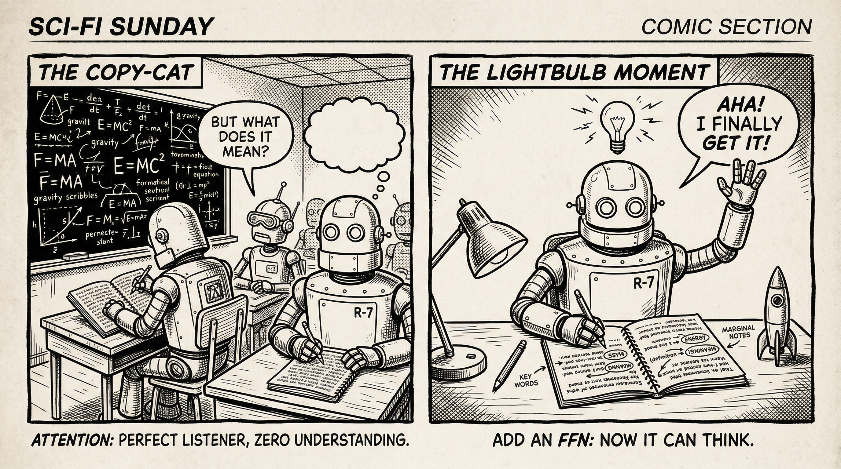
Attention has just run on “The cat sat.” The word “sat” now carries blended context from “The” and “cat.” It knows the subject is a cat and the sentence is past tense. But what can it do with that knowledge?

If we skip straight from attention to the output layer, the model can only produce weighted combinations of existing token representations. It can copy and blend, but it can’t compute anything new. It couldn’t combine “subject is singular” + “verb should agree” into a grammatical prediction. It couldn’t learn “after [animal] [past-tense verb], predict a location.” It needs a processing step.

That processing step is the Feed-Forward Network: per-token computation that transforms gathered context into useful features.

• Attention = “gather information from other tokens” (communication)
• FFN = “think about what you’ve gathered” (computation)

Step through the animation to see how the FFN processes a single token’s vector:

What to look for: The vector expands to 4x its size, giving ReLU room to create sparse activation patterns (about half the neurons fire). Then it contracts back to the original size. Same shape in, same shape out, but the values have been transformed.

The FFN applies two linear transformations with ReLU in between. ReLU is the simplest non-linear activation: negative values become 0, positive values pass through unchanged.

Why expand then contract? ReLU makes a binary decision on each dimension: keep (positive) or kill (zero). Each dimension is one yes/no question about the input. With only 512 dimensions, you get 512 questions. With 2048 dimensions, you get 2048 questions. More questions means finer-grained analysis, the same reason 20 Questions works better than 5 Questions. (Unlike 20 Questions, the FFN’s “questions” aren’t sequential or adaptive: all 2048 ReLU decisions happen simultaneously and independently, without building on each other’s answers.)

Here’s a tiny worked example. Say the input is [1.0, -0.5] and we expand to 4 dims:

A different input, say [-0.5, 1.0], would trigger different neurons to fire, producing a completely different pattern. With 4 neurons, there are up to $2^4 = 16$ possible on/off combinations, so the network can treat up to 16 different input regions differently. With only 2 neurons (no expansion), you’d get just $2^2 = 4$ regions. In the real model: $2^{2048}$ possible patterns vs $2^{512}$ without expansion. Exponentially more expressive.

Why contract back? The expansion is temporary scratch space. The rest of the model (attention in the next block, the output layer) expects 512-dim vectors. The contraction reads the ReLU activation pattern and writes a 512-dim summary of what was detected.

The FFN has more parameters than the attention layers in each block: roughly twice as many. Most of a transformer’s weights live in FFN layers, not attention. (Here, $d_{\text{model}}$ is the vector size that flows through the entire transformer: 512 in the original paper, 8 in our toy model. $d_{ff}$ is the expanded FFN width, typically $4 \times d_{\text{model}}$.)

class FeedForward:
    def __init__(self, d_model, d_ff):
        self.W1 = np.random.randn(d_model, d_ff) * 0.01
        self.b1 = np.zeros(d_ff)
        self.W2 = np.random.randn(d_ff, d_model) * 0.01
        self.b2 = np.zeros(d_model)

    def forward(self, x):
        # Expand -> ReLU -> Contract
        hidden = np.maximum(0, x @ self.W1 + self.b1)  # ReLU
        return hidden @ self.W2 + self.b2

Anatomy of a Transformer Block

Now we have both pieces: attention for communication and FFN for computation. But stacking them naively fails. Each sub-layer completely overwrites its input: the attention output replaces the original token vector, then the FFN output replaces that. After 96 blocks, nothing remains of the original signal. Gradients face the same problem in reverse: they must pass through every transformation, shrinking toward zero. Two helpers fix this:

• Residual connection: add the sub-layer’s input back to its output ($x + \text{sublayer}(x)$). The original signal always passes through, even if the sub-layer learns nothing useful. Gradients get a clean shortcut that bypasses the transformation entirely. (Forgot why? Review residual connections.)
• Layer normalization: normalize the vector to mean $\approx$ 0 and std $\approx$ 1, preventing activations from drifting or exploding across layers. (Forgot why? Review LayerNorm.)

Where you place LayerNorm matters. The original 2017 paper put it after the residual add (Post-LN). This worked for 6 layers, but when researchers tried stacking to 96, training became unstable: gradients had to pass through LayerNorm at every layer on the residual path, and the repeated scaling caused them to vanish. The fix was simple: move LayerNorm before the sub-layer (Pre-LN), so the residual path stays a clean identity with nothing blocking gradient flow. Today, Pre-LN is the default (GPT-2, GPT-3, LLaMA).

The diagram below shows the Pre-LN layout. Toggle to Post-LN to see how the order changes. Click any block for details. (The “Want to Go Deeper?” section at the bottom of this page has an animated gradient flow comparison.)

What to look for: Data flows top to bottom through two sub-layers (Gather and Think). Each sub-layer has the same pattern: normalize, transform, add back. The dashed arcs on the right carry the original signal around each transformation.

class TransformerBlock:
    def __init__(self, d_model, n_heads, d_ff):
        self.attn = MultiHeadAttention(d_model, n_heads)
        self.ffn = FeedForward(d_model, d_ff)
        self.ln1 = LayerNorm(d_model)
        self.ln2 = LayerNorm(d_model)

    def forward(self, x, mask=None):
        # Sub-layer 1: Attention
        x = x + self.attn(self.ln1(x), mask)

        # Sub-layer 2: FFN
        x = x + self.ffn(self.ln2(x))

        return x

Worked Example: One Token Through a Block

Trace the word “sat” (from “The cat sat”) through a single transformer block. Step through each operation to see how the vector transforms (4-dim vectors for simplicity):

What to look for: The attention and FFN outputs are small nudges, not dramatic rewrites. The residual adds preserve most of the original signal. After both sub-layers, the output has the same shape as the input but carries richer information. This output feeds into the next block, which repeats the same gather-then-think pattern. A typical model stacks 12 to 96 blocks deep. (Why do we need residual connections at all? They keep gradients healthy in deep networks. Full explanation here.)

The Three Transformer Variants

A single transformer block can process any sequence. But different tasks have different constraints. Translation needs to read a full sentence before writing the output. Text generation must work left-to-right, never peeking ahead. Sentence classification needs to see the whole input at once. One architecture can’t optimally serve all three. The choice comes down to a single constraint: which tokens can attend to which?

What to look for: Click “sat” in both matrices. In the bidirectional matrix (encoder), “sat” attends to all 6 tokens, including “on”, “the”, “mat” that come after it. In the causal matrix (decoder), “sat” can only see itself and the two tokens before it. The blocked cells (x) are set to negative infinity before softmax, giving them zero weight. This single constraint is what separates the three variants.

Encoder-Decoder (Original Transformer, T5, BART)

The original 2017 “Attention Is All You Need” architecture uses both columns: an encoder to read the input and a decoder to generate the output.

How it works: The encoder processes the full input with bidirectional self-attention: every word sees every other word. It produces a set of context-rich representations. The decoder generates output one token at a time using causal self-attention (can only see previous output tokens), plus cross-attention that reads from the encoder’s representations.

Cross-attention is the bridge: the decoder’s queries ask “what part of the input do I need right now?”, and the encoder’s keys and values provide the answer.

What to look for: Click each French token. “chat” attends 85% to “cat”, “assis” to “sat”, “Le” to “The”. The model learns this alignment from training data alone, without explicit word-pairing rules. (Forgot cross-attention? Review it here.)

Best for: Tasks where input and output are different sequences: translation, summarization, speech-to-text. T5 showed this architecture works for almost any NLP task by framing it as text-to-text.

Encoder-Only (BERT)

What if you don’t need to generate text at all? Drop the decoder, keep only the encoder stack.

How it works: Every token sees every other token through bidirectional self-attention. There’s no causal mask, no generation. The model reads the entire input simultaneously and produces contextualized representations for each token.

This matters for understanding tasks. Consider the word “bank” in two sentences: “I sat by the river bank” vs “I went to the bank to deposit money.” A bidirectional model sees “river” to the right and resolves the ambiguity. A causal model processing left-to-right would have to guess without seeing what comes after.

The [CLS] trick: BERT prepends a special [CLS] token to every input. After passing through all layers, this token’s representation captures a summary of the entire sequence. For classification tasks (sentiment, spam detection), you just feed [CLS]’s final vector through a linear layer and softmax.

The [MASK] trick: During training, BERT randomly replaces ~15% of tokens with [MASK] and learns to predict the original. This “fill in the blank” objective (masked language modeling) forces the model to build deep bidirectional understanding. Deep dive into BERT.

Best for: Classification, named entity recognition, sentence similarity, question answering (extractive).

Limitation: Cannot generate text. There’s no autoregressive mechanism, no way to produce one token at a time.

Decoder-Only (GPT, LLaMA, Claude)

The simplest design: just the decoder stack, no encoder, no cross-attention. One job: predict the next token.

Step through the animation below. At each position, the model can only see the tokens before it (causal attention), and it predicts what comes next:

What to look for: At position 1, “The” is all the model has, and it guesses “cat.” At position 2, it sees “The cat” and guesses “sat.” Each step adds one more token of context. The curved arrows show which tokens are visible to the current position: always a growing left-to-right window, never peeking ahead. During training, all four positions are computed in parallel (the causal mask blocks future tokens). During generation, they happen one at a time.

“Decoder-only”? But it clearly understands input. The name is confusing, and Karpathy has argued that “autoregressive transformer” would be more accurate. Step through the animation below to see where the name comes from:

The model absolutely builds rich representations of its input (it “encodes” in the everyday sense), but architecturally its building block descends from Vaswani’s decoder column, not the encoder. The name is about lineage, not capability.

Why it won: Three reasons:

1. Simplicity. No encoder-decoder boundary, no cross-attention. One uniform stack of blocks. Fewer design choices means fewer things to get wrong.

2. Scaling. Decoder-only models scale predictably: more parameters, more data, better performance. The scaling laws discovered by Kaplan et al. (2020) showed smooth, power-law improvements across many orders of magnitude.

3. Emergent abilities. Next-token prediction turns out to be a surprisingly general objective. To predict what comes next in text, the model must learn grammar, facts, reasoning, and even some degree of world knowledge. GPT-3 showed that a large enough decoder-only model can do translation, summarization, and question answering without being specifically trained for them: just provide a few examples in the prompt (few-shot learning).

Deep dive into GPT.

Computation Cost

Every token must attend to every other token. That means the attention matrix has $n^2$ entries, and the cost grows quadratically with sequence length. Click through the sequence lengths below to feel the blowup:

What to look for: Start at 512 tokens (our baseline), then click through to 128,000. At true scale, the first two bars are invisible compared to the last one. Toggle log scale to see all four, then switch back to true scale to feel the real gap. Going from 512 to 128,000 tokens means 62,500x more computation in the attention layer alone.

This quadratic cost is why long-context models are expensive, and why researchers developed efficient attention variants: Flash Attention (exact attention with better memory access patterns), sliding window attention (Mistral, attend to a local window only), and linear attention approximations.

The FFN is cheaper per token ($O(n \cdot d \cdot d_{ff})$, linear in sequence length) but uses more parameters. Embedding lookup is trivially cheap ($O(n)$).

Quick Summary

Next: Training

You understand the architecture: what each component does and how they fit together. But a freshly initialized transformer produces random noise. How does it learn? Training →