Training
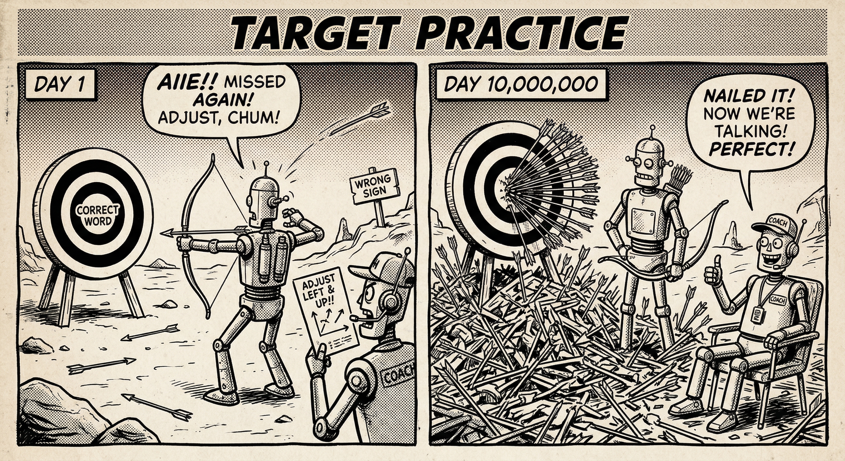
You’ll learn how transformers train by predicting the next token at every position in parallel. You’ll also see how cross-entropy loss, teacher forcing, backpropagation, residual connections, and optimizer updates turn wrong guesses into better weights.
You’ve seen the architecture: attention gathers context, the FFN processes it, residual connections and layer norm keep things stable. But a freshly initialized transformer has random weights. Ask it to complete “The cat sat on the” and it might say “purple” or “seventeen.” Every weight is noise, and every prediction is a coin flip across a 50,000-word vocabulary. The model needs a signal telling it how wrong it is at every position, millions of times over, until the noise becomes language.
The Training Objective: Next-Token Prediction
The learning process boils down to one objective: given all previous tokens, predict the next one. Think of it as a fill-in-the-blank test where every position in the sentence is a blank, and the model is graded on all of them simultaneously. It turns out that mastering next-token prediction, at scale, teaches a model grammar, facts, reasoning, and even code. Why? Because to predict well across all domains, the model must learn what words mean and how they relate to each other.
Given all previous tokens, predict the next one.
The model decomposes the probability of a full sentence into a chain: the probability of each word given all the words before it.
Train Together, Generate One at a Time
Play the 3 rounds below to compare parallel training with one-by-one generation:
The Loss Function
How do we tell the model how wrong it is? We need a single number that says “your prediction was this far off.” Drag the dot on the curve below to see how that number behaves:
Cross-Entropy Loss
P(correct) = 50% loss = 0.69Drag anywhere on the chart. Low probability on the correct token (left) means huge loss. High probability (right) means tiny loss. The penalty grows explosively as probability drops toward zero.
What to look for: Drag the dot to 1% and watch the loss shoot past 4. Drag it to 90% and the loss is barely 0.1. The curve is not a straight line: the penalty for being almost certain and wrong is dramatically worse than being slightly uncertain. The two reference points show where an untrained model (8%, loss 2.53) and a trained model (70%, loss 0.36) sit on the curve.
This is cross-entropy loss: the negative log of the probability the model assigned to the correct next token. Here’s a concrete example. The model predicts after “The cat sat on the”:
| Candidate | Model’s probability | Correct? |
|---|---|---|
| “mat” | 8% | ✓ |
| “floor” | 12% | |
| “bed” | 10% | |
| “table” | 7% |
The loss at this position: . That’s a strong penalty, because the model wasn’t very confident about the right answer. If it had assigned 70% to “mat,” the loss would be just . You can verify both on the interactive curve above.
The total loss averages this across all positions in the sequence.
Teacher Forcing
If we train the model on its own predictions and it makes a mistake early, that error cascades. Step through the comparison below to see how one wrong prediction at position 1 snowballs:
Teacher Forcing vs Free-Running
Position 1: predict "cat"Both modes see the same input and make the same (wrong) prediction: "dog" instead of "cat." With teacher forcing, this mistake won't affect the next position.
What to look for: At position 1, both tracks are identical. By position 3, the free-running track has drifted to a completely different sentence. By position 5, four of five context tokens are wrong (red), and the model is learning from garbage. Teacher forcing stays clean at every step because it always uses the ground-truth context.
Teacher forcing means: at each position, always feed the correct previous tokens as context, even if the model’s last prediction was wrong. Think of it as studying with an answer key: you see the correct answer to the previous problem before moving to the next one, so you never have to recover from your own mistakes. (Unlike a real answer key, the model never practices recovering from errors during training, so at inference time it encounters input patterns it never saw. This gap is called exposure bias.)
| Context used | Risk | |
|---|---|---|
| Teacher forcing | Always real tokens | None (clean signal) |
| Free-running | Model’s own predictions | Errors compound at every step |
In practice, models trained with teacher forcing still generate well, because each position learned from a clean signal. The exposure bias gap turns out to be small enough that it rarely causes problems at scale.
The Training Loop
Training follows the standard deep learning cycle. Step through the visualization below to see each phase with concrete numbers:
Training Step Walkthrough
Predicted probability distributions at all 5 positions.
What to look for: Step through all four phases. Each position predicts its next token, and the loss measures how much probability went to the correct answers. Backpropagation computes how each parameter affects that loss. The animation illustrates an update that improves every position; in a real batch, shared parameters can help some predictions and hurt others. Track the average training loss and a separate validation loss over many updates.
The four steps in every training iteration:
| Step | What Happens |
|---|---|
| Forward pass | Run all tokens through the model in parallel, get predictions at every position |
| Compute loss | Cross-entropy between each prediction and its target, then average |
| Backward pass | Compute gradients via backpropagation (how much each weight contributed to the error) |
| Update weights | Optimizer nudges parameters to reduce the loss |
Backpropagation: How Error Becomes Learning
The loss tells us how wrong the model is. Backpropagation tells us who’s responsible. For each of the model’s millions of weights, we need to answer one question: “If this weight were slightly larger, would the loss go up or down, and by how much?” That answer is the gradient, and computing it for every weight is what backpropagation does.
Passing Blame Backward
The model is a chain of operations: embedding → attention → FFN → layer norm → attention → FFN → … → output projection. To find each weight’s gradient, backpropagation works backward from the loss, asking each layer: “How much did your output change when your input changed?” Then it multiplies these local effects together. This is the chain rule of calculus applied one layer at a time.
A concrete example: in the Training Loop visualization above (Step 3), position 4 has the highest loss because the model predicted “floor” instead of “mat.” Backpropagation traces this error backward:
- Output layer: “Increase the logit for ‘mat,’ decrease it for ‘floor’”
- Final FFN: Adjust the weights that would have boosted the “mat” representation in this context
- Final attention layer: The attention weights that chose which earlier positions to focus on get adjusted, so the model attends more to “sat on” (which strongly predicts “mat”)
- Earlier layers: Smaller adjustments ripple back, each refining how the model represents this input pattern
- Embeddings: Even the token embeddings get a tiny nudge, adjusting what “on” and “the” mean to the model
Step through the full forward and backward pass for this example:
Forward & Backward Pass
Forward →Each token is converted to a dense vector. These vectors are the model's starting representation of each word.
What to look for: In the forward phase (steps 1-4), watch data flow left to right through the pipeline, ending at a loss of 1.77. Then in the backward phase (steps 5-8), gradients flow right to left. At steps 6 and 7, notice how the residual connection splits the gradient into two paths: one through the layer (updating weights) and one through the skip connection (preserving signal strength). By step 8, even the earliest embeddings receive a gradient.
All five positions do this simultaneously. Their gradients are summed to produce one set of weight updates for the whole model.
Why Transformers Don’t Have Vanishing Gradients
If you’ve seen RNN backpropagation, you know the problem: gradients flow through every timestep sequentially, getting multiplied by the same weight matrix at each step. After enough multiplications, the signal shrinks to near zero. The model can’t learn long-range dependencies. (See Vanishing Gradients for the full story.)
Transformers avoid this in two ways:
- No temporal unrolling. Every position computes its prediction independently, so there’s no chain of timesteps to propagate through. Position 1’s gradient doesn’t need to flow through positions 2, 3, 4, 5.
- Residual connections create gradient highways. The residual connection has a gradient of just 1 through the addition. Even if a layer’s internal gradients are small, the skip-connection path carries the error signal to earlier layers at full strength. This is why transformers can stack 96+ layers without gradients vanishing.
Toggle between the two modes below to see the difference. Then try increasing the layer count:
Gradient Flow Through Layers
Toggle modes and drag the slider to add layers. Real transformers stack 12 to 96+ layers, making residual connections essential.
What to look for: With residuals, every bar stays near 1.0, even at the bottom. Switch to “Without” and watch the bars shrink layer by layer. Increase to 12 layers: with residuals the bars barely change, but without them the embedding gradient drops to near zero. This is why deep transformers require residual connections.
| RNN | Transformer | |
|---|---|---|
| Gradient flow | Sequential through time (BPTT) | Parallel across positions |
| Vanishing risk | High (same matrix reused at each step) | Low (residual connections) |
| Practical depth | ~5-10 layers | 96+ layers |
Optimization
Gradients point each weight in the right direction, but how far should it move? Three problems arise with a naive approach (plain gradient descent with a fixed step size):
- One size doesn’t fit all. Some parameters need large updates, others need tiny nudges. A single learning rate can’t serve both.
- Gradients are noisy. Each batch is a small sample of the data. One batch might push a weight left; the next pushes it right. Following every fluctuation wastes steps.
- Weights can grow unchecked. Without a constraint, some weights balloon to extreme values, and the model memorizes the training data instead of learning general patterns.
AdamW solves all three. It’s the standard optimizer for transformer training:
- Adaptive learning rates per parameter. Parameters with historically large, volatile gradients get smaller steps (to avoid overshooting). Parameters with consistently small gradients get larger steps (to make faster progress). Each of the model’s millions of parameters gets its own effective step size.
- Momentum smooths out noise by averaging gradients over recent steps. One bad batch can’t throw the optimizer off course, just like averaging poll results is more reliable than any single poll.
- Weight decay adds a gentle pull toward smaller weights at every step. This prevents overfitting by discouraging any single weight from growing too large. (Unlike classic L2 regularization, AdamW applies decay directly to the weights, not to the gradients, which turns out to generalize better.)
Learning Rate Schedule
Even with AdamW’s per-parameter adaptation, the global learning rate follows a planned schedule. Drag across the chart to see how it changes over 100,000 training steps:
Learning Rate Schedule
Step 30k LR 5.0e-4 Cosine DecayDrag anywhere on the chart. The warmup ramp (first 4k steps) prevents wild updates from noisy early gradients. Cosine decay smoothly reduces the rate for fine-grained convergence.
What to look for: Drag to the far left and watch the learning rate ramp from zero during warmup (the first ~4,000 steps). Then drag right and watch cosine decay smoothly bring it back down. At step 50k, the rate is about half its peak. By 100k, it’s near zero. The shape is the key: ramp up fast, come down slow.
| Phase | What Happens | Why |
|---|---|---|
| Warmup (~4,000 steps) | Linearly ramp LR from 0 to peak | Early gradients are noisy and AdamW’s momentum estimates haven’t stabilized; large steps would destabilize training |
| Peak | Maximum learning rate (e.g., 6×10⁻⁴) | Fastest learning, once gradient statistics are reliable |
| Cosine decay | Smoothly decrease following cos(x) to near 0 | Fine-grained convergence as the model approaches optimal weights |
The Full Training Pipeline
This table describes training at a large scale. Your first experiment in Train Your Own GPT uses a small bundled corpus, a character vocabulary, and a short training run. It also holds out validation text before making training windows, so you can measure performance on text the optimizer never sees.
| Step | Action |
|---|---|
| 1 | Collect massive text corpus (books, web, code…) |
| 2 | Tokenize entire corpus (BPE with ~50K vocabulary) |
| 3 | Split into batches of sequences (e.g., 2048 tokens each) |
| 4 | For each batch: forward, loss, backward, update |
| 5 | Repeat for millions of steps |
| 6 | Result: a model that can predict next tokens |
Quick Summary
| Concept | What Happens | Intuition |
|---|---|---|
| Next-token prediction | At every position, predict the next token | One simple objective that teaches everything |
| Cross-entropy loss | Confident and wrong = huge penalty | |
| Teacher forcing | Always use real tokens as context | Study with the answer key, not your own mistakes |
| Backpropagation | Chain rule traces error backward through every layer | Blame assignment: who caused the mistake? |
| Training loop | Forward, loss, backward, update | Standard gradient descent, at enormous scale |
| LR schedule | Warmup, peak, cosine decay | Start gentle, go fast, then fine-tune |
- I can explain the next-token prediction objective and why all positions train in parallel
- I understand cross-entropy loss and why confident-but-wrong predictions are penalized most
- I understand teacher forcing and why it prevents error compounding
- I can describe the four steps of the training loop: forward, loss, backward, update
- I can explain how backpropagation computes gradients and why residual connections are essential for deep transformers
- I know what exposure bias is (the mismatch between teacher forcing and free-running inference)
Next: Inference
The model is trained. How does it actually generate text, one token at a time? Inference →