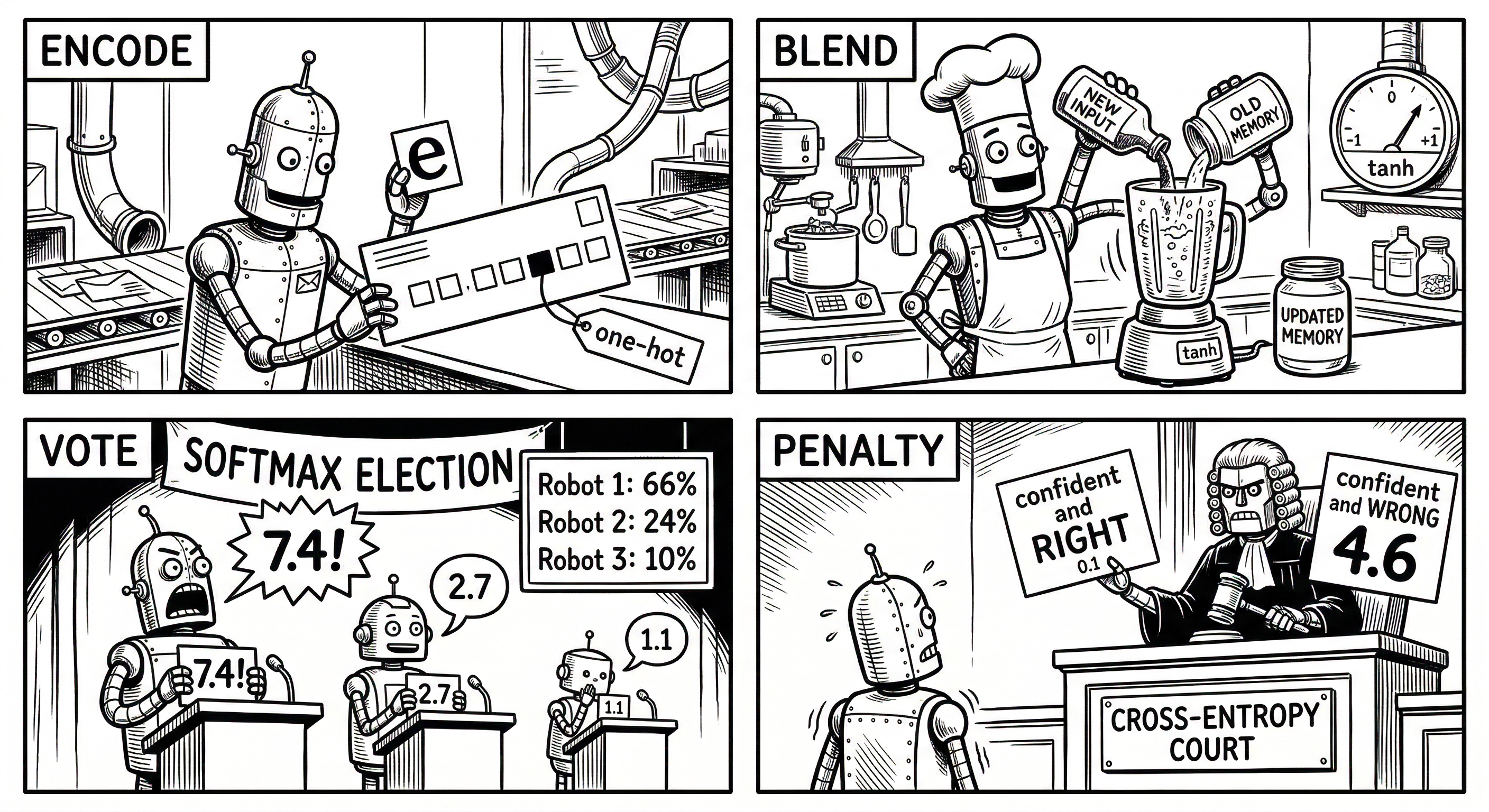
You’ll learn how an RNN turns inputs into one-hot vectors, blends each input with the previous hidden state, and produces a prediction. You’ll also see how softmax turns scores into probabilities and how cross-entropy loss grades those predictions.
In the Introduction, we learned what an RNN does: it processes sequences while maintaining memory. Now let’s see how it actually computes predictions, step by step.
Watch the Forward Pass First
Before we break anything down, watch it work. Step through each word and see how the hidden state (memory) updates and predictions shift:
🧠
RNN Step-by-Step
Watch how memory builds as each word is read
→→→
Memory before
Empty — nothing read yet
memory pattern
reads "I"
↓
mix old memory + new word, then compress
↓
Memory after
"I"
updated pattern
💬First word: "I". The memory activates for the first time, but with just one word the predictions are spread thin.
🎯 Next word prediction:
"love"
30%
"my"
26%
"dog"
24%
Step 1 of 4
What to look for: Step through the words one at a time. Watch the hidden state “fingerprint” (the colored dots) change after each word as the network blends new input with old memory. Notice how the prediction bars reshuffle at every step: after “I,” many next-words are plausible; after “I love my,” the distribution narrows sharply toward pets and family.
Now let’s break down what happens at each stage.
Step 1: Encoding the Input
Computers don’t understand words — they understand numbers. So we first convert each character or word into a vector.
One-Hot Encoding
The simplest approach: a vector of all 0s except for a single 1 at the position of our character.
If our vocabulary is ['a', 'b', 'c', 'd']:
‘a’ → [1, 0, 0, 0]
‘b’ → [0, 1, 0, 0]
‘c’ → [0, 0, 1, 0]
‘d’ → [0, 0, 0, 1]
The vector has exactly one “hot” (1) element — hence the name one-hot encoding.
Step 2: Updating the Hidden State
This is the core of an RNN. The network combines two things:
What it just saw — the current input
What it remembers — the previous hidden state
Think of it like a blender: you pour in the new ingredient (current input) and the old smoothie (previous memory), blend them together, and get a new smoothie (updated memory). The blending recipe is what the network learns during training.
Let’s trace through a concrete example. Imagine processing “to be” and we just reached the letter 'e':
Ingredient
What it contributes
Intuition
Current input
”What signal does 'e' carry?”
The new ingredient
Previous memory
”What did we learn from 'to b'?”
The old smoothie
Bias
Learned offset, adds flexibility
A pinch of salt
Squashing (tanh)
Keeps values in [-1, 1] so they don’t explode
The blender’s speed limit
Why squash the result? Without it, each step multiplies values by weight matrices — they’d grow or shrink without bound. The squashing function is a “pressure valve”: no matter what’s fed in, the output stays between −1 and 1.
The hidden state update equation:
ht=tanh(Wxh⋅xt+Whh⋅ht−1+bh)
The subscripts tell you what each weight matrix connects:
Wxh = weights from x (input) to h (hidden) — shape: (hidden_size, vocab_size)
Whh = weights from h (hidden) to h (hidden) — shape: (hidden_size, hidden_size)
bh = bias for the hidden layer — shape: (hidden_size,)
Why two separate weight matrices? One processes “what am I seeing now?” (Wxh⋅xt) and the other processes “what do I remember?” (Whh⋅ht−1). Their results are added together — the network learns how to balance new input vs. memory.
✍️Fill in the Blanks
The hidden state is computed by combining the input with the hidden state, then applying a non-linear activation.
Fill in every blank, then check your answer.
A blank is still empty.
Fill in every blank before checking your answer.
Not quite.
Try another answer, or reveal the solution.
Correct.
One accepted answer is shown in each blank.
Answer revealed.
The blanks now show the answers.
Step 3: Computing Output Probabilities
Now we turn the hidden state into a prediction: “What’s the most likely next character?”
Raw Scores (Logits)
First, we compute one raw score per vocabulary item. These raw scores are called logits — they can be any real number, positive or negative. Higher score = network thinks that character is more likely. But they’re not yet probabilities — they don’t sum to 1.
Softmax: From Scores to Probabilities
We need to convert logits into proper probabilities. You might think: “just divide each score by the total.” But that fails with negative scores. Softmax solves this — think of it as an election where confident voters shout louder:
Every score gets exponentiated — this makes everything positive, and amplifies differences
Then we divide by the total so everything sums to 1
The gap between 2.0 and 1.0 in logit space becomes a 2.7x gap in probability space — softmax amplifies differences.
Logits from a linear projection of the hidden state:
yt=Why⋅ht+by
Softmax converts logits to probabilities:
pi=∑jeyjeyi
Why exponential, not just dividing by the sum?
ex is always positive — no negative probabilities
ex grows rapidly — amplifies small differences in logits
Dividing by the total ensures everything sums to 1
🤔Quick Check
If the logits before softmax are [2.0, 1.0, 0.1], which statement is true about the softmax output?
Your turn
Choose an answer to check your understanding.
Try another option
Think about what happens when you exponentiate different values...
Correct!
Softmax uses exponentials: e^2.0 ≈ 7.4, e^1.0 ≈ 2.7, e^0.1 ≈ 1.1. The probabilities are roughly [0.66, 0.24, 0.10]. The gap between 2.0 and 1.0 in logit space becomes a 2.7× gap in probability space — softmax amplifies differences, making the model 'more confident' about its top choice.
Answer: B
Softmax uses exponentials: e^2.0 ≈ 7.4, e^1.0 ≈ 2.7, e^0.1 ≈ 1.1. The probabilities are roughly [0.66, 0.24, 0.10]. The gap between 2.0 and 1.0 in logit space becomes a 2.7× gap in probability space — softmax amplifies differences, making the model 'more confident' about its top choice.
Attempts: 0
Step 4: Measuring the Error (Loss)
How do we know if our prediction was good? We need a loss function — a single number that says “how wrong was the model?”
We use cross-entropy loss — it takes the probability the model assigned to the correct answer and applies negative log. Think of it as a confidence penalty:
Predicted correctly with probability 0.9 → loss = 0.10 — low, well done
Predicted correctly with probability 0.01 → loss = 4.6 — huge penalty!
The key property: being confidently wrong is punished far more than being slightly uncertain. This is exactly what we want — the model should never be confident and wrong.
Cross-entropy loss at timestep t:
Lt=−log(pt[target])
Why negative log?
When p≈1 (correct and confident): −log(1)=0 — zero loss, perfect
When p≈0 (wrong): −log(0.001)=6.9 — huge penalty
The log creates an asymmetric punishment: being confidently wrong is punished exponentially more
The total loss sums across all timesteps:
L=∑tLt=−∑tlog(pt[targett])
Here’s the full algorithm. Notice the numerically stable softmax (subtract max before exponentiation):
def forward_pass(inputs, targets, h_prev):
    """
    Process a sequence and compute loss.

    Args:
        inputs:  List of character indices [t0, t1, ...]
        targets: List of target indices, shifted by 1
        h_prev:  Initial hidden state (hidden_size x 1)

    Returns:
        loss:   Total cross-entropy loss
        cache:  Intermediate values needed for backprop
    """
    xs, hs, ys, ps = {}, {}, {}, {}
    hs[-1] = h_prev
    loss = 0

    for t in range(len(inputs)):
        # Step 1: One-hot encode input
        xs[t] = np.zeros((vocab_size, 1))
        xs[t][inputs[t]] = 1

        # Step 2: Update hidden state
        hs[t] = np.tanh(Wxh @ xs[t] + Whh @ hs[t-1] + bh)

        # Step 3: Compute output logits
        ys[t] = Why @ hs[t] + by

        # Step 4: Numerically stable softmax
        shifted = ys[t] - np.max(ys[t])
        ps[t] = np.exp(shifted) / np.sum(np.exp(shifted))

        # Step 5: Accumulate cross-entropy loss
        loss += -np.log(ps[t][targets[t], 0] + 1e-8)

    return loss, (xs, hs, ys, ps)
🤔Quick Check
In the forward pass, why do we store all the intermediate values (xs, hs, ys, ps)?
Your turn
Choose an answer to check your understanding.
Try another option
Think about what happens after the forward pass...
Correct!
We need these cached values during backpropagation! The gradients at each timestep depend on the activations computed during the forward pass. This is why RNNs use more memory for longer sequences.
Answer: B
We need these cached values during backpropagation! The gradients at each timestep depend on the activations computed during the forward pass. This is why RNNs use more memory for longer sequences.
Attempts: 0
Explore the Computation Graph
Ready to go deeper? This interactive graph lets you inspect every single node — one-hot vectors, weight matrix multiplications, hidden states, logits, and softmax outputs — as the RNN processes a sentence character by character:
RNN Computation Graph
Forward
vectorsmatricesopsactivations
100%
V=0H=4L=—
What to look for:
x (red): One-hot encoded inputs, sparse vectors with a single 1
h (green): Hidden states, updated at every timestep
y and p (blue): Output logits (y) and final softmax probability distributions (p)
W (yellow) and b (indigo): Shared weight matrices and bias vectors reused across all timesteps
Quick Summary
Step
What happens
Intuition
1. Encode
Convert input to one-hot vector
Give the character an address in vocabulary space
2. Update
Blend input + memory through squashing
New ingredient + old smoothie = updated smoothie
3. Output
Compute raw scores (logits)
“How likely is each character?“
4. Softmax
Convert scores to probabilities
Election: confident voters shout louder
5. Loss
Measure prediction error
Confidence penalty: being wrong and sure is expensive
Numerical Stability in Softmax
The raw softmax formula can silently overflow when logits are large (e.g., e1000=∞). The fix is to subtract the max before exponentiation:
shifted = y - np.max(y) # safe: largest value becomes 0p = np.exp(shifted) / np.sum(np.exp(shifted))
Subtracting the max doesn’t change the final probabilities (the constant cancels in the division) but prevents floating-point overflow.
Why Cross-Entropy?
Cross-entropy has three properties that make it ideal for classification:
Simple gradient: ∂yi∂L=pi−1i=target — just subtract 1 from the target’s probability
Punishes confident wrong answers: Being 99% sure of the wrong answer is penalised far more than being 51% sure
Probabilistic grounding: Minimising cross-entropy is equivalent to maximising the likelihood of the training data
Truncated Backpropagation Through Time
For very long sequences (an entire book), backpropagating through every single timestep is impractical. Instead:
Process a chunk (e.g., 100 characters)
Compute gradients for that chunk only
Move to the next chunk, carrying the hidden state forward
The hidden state preserves context across chunks, but gradients only flow within each chunk. This trades a small amount of gradient accuracy for a dramatic reduction in memory.
Temperature Sampling
When generating text (not training), we can control creativity with temperature τ:
pi=∑jeyj/τeyi/τ
τ<1: Sharpens the distribution — more confident, less varied output
τ>1: Flattens the distribution — more random, more creative output
τ→0: Always picks the single highest-probability token (greedy decoding)
Key References
The original RNN forward pass. Elman, “Finding Structure in Time” (1990) defined the simple recurrent network: feed the previous hidden state back as input alongside the current token. The hidden state update equation on this page (ht=tanh(Wxh⋅xt+Whh⋅ht−1+bh)) is exactly the Elman network.
min-char-rnn. Karpathy, “The Unreasonable Effectiveness of Recurrent Neural Networks” (2015) walked through a minimal character-level RNN in ~100 lines of Python. The implementation on this page follows the same structure. The blog post remains one of the best introductions to RNNs in practice.
I can explain what a one-hot vector is and why its size equals the vocabulary size
I understand how the hidden state combines new input with previous memory
I know why tanh is used as the activation function (keeps values bounded)
I can trace through the softmax computation and explain why it uses exponentials
I understand cross-entropy loss and why confident wrong predictions are heavily penalized
Next Steps
You now know exactly how an RNN makes predictions. But how does it learn — how do the weights get tuned? Next up: Backward Pass & BPTT →, where gradients flow backwards through the sequence to update every parameter.