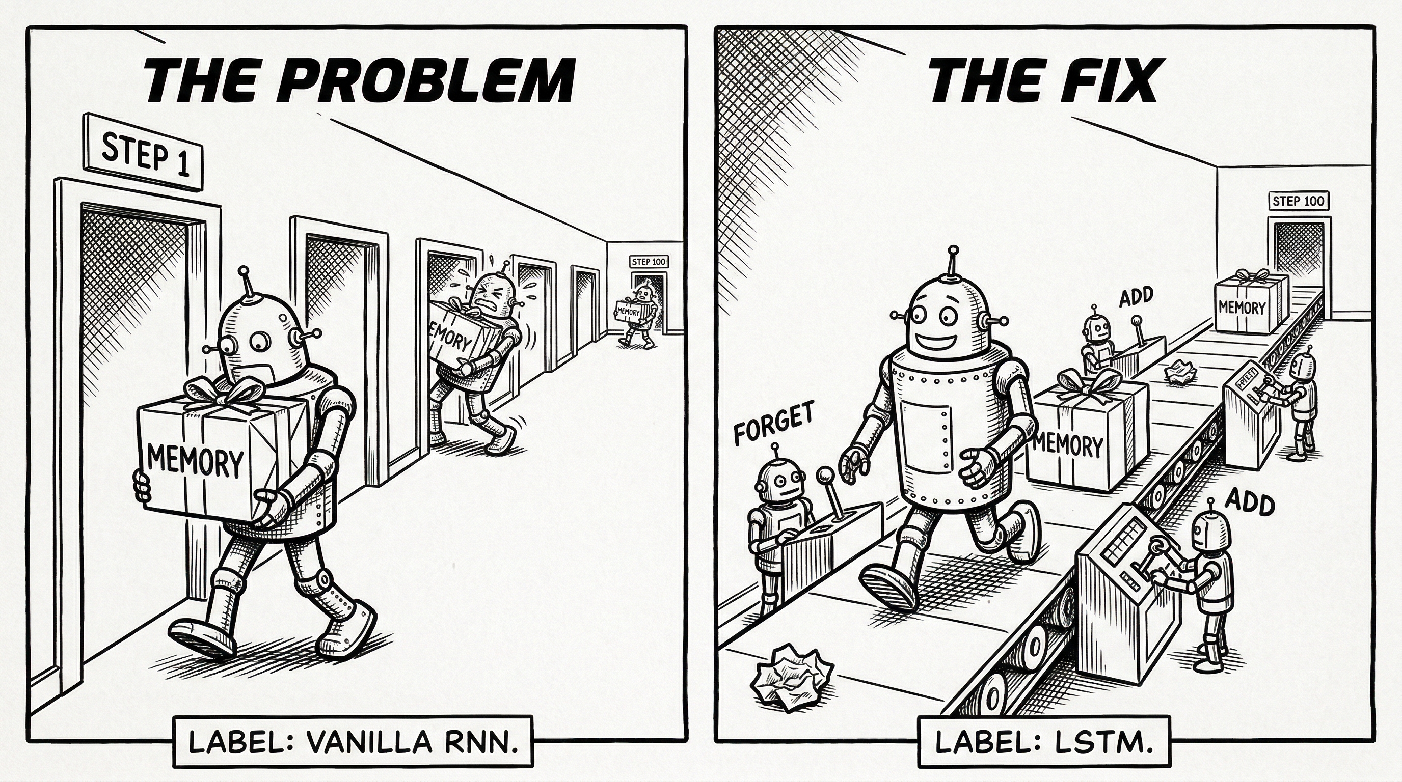
You’ll learn why repeated multiplication makes RNN gradients vanish or explode across long sequences, and why that blocks long-range learning. You’ll also see how LSTMs and GRUs preserve information with gates, and why transformers avoid the same bottleneck with direct token-to-token connections.
In the backward pass, we saw how gradients flow through time via repeated multiplication by WhhT. Now we’ll see why this causes a fundamental problem — and the elegant architectural solutions that fix it.
The Problem
Train an RNN on long sequences and plot gradient magnitude at each timestep:
Gradient Magnitude Through Time
||dh|| (log)
6e-3
0
8e-3
0.01
2
0.01
0.02
4
0.02
0.03
6
0.04
0.05
8
0.07
0.09
10
0.12
0.15
12
0.20
0.26
14
0.34
0.45
16
0.59
0.77
18
1.0
19
Timestep (t)
Gradients decaying: With |λ| = 0.90, gradients shrink to 0.006 at t=0. Short sequences work, but long-range dependencies are hard to learn.
What to look for: The bars represent gradient magnitude at each timestep. Notice how bars on the left (early tokens) are dramatically smaller than the right (near the loss). The gradient doesn’t just decrease, it drops exponentially. By t=0, almost no learning signal remains.
Try it yourself: Drag the |λ| slider below 0.9 to see gradients vanish, or above 1.2 to see them explode. Then increase the sequence length T to see how the problem gets worse with longer sequences.
Consequence: early tokens don’t learn. The network can’t capture long-range dependencies. A word at the start of a sentence has almost no influence on the loss at the end.
Why Gradients Vanish
The Core Intuition
Each backward step through time multiplies the gradient by a factor. Think of it like a game of telephone: the message (gradient) gets distorted at every step. If each step slightly shrinks the signal, after enough steps the message is gone entirely.
When you repeatedly multiply a number by a constant, the result grows or shrinks exponentially. Multiplying by 0.9 a hundred times: 0.9100≈0.00003. Multiplying by 1.1 a hundred times: 1.1100≈13,780.
The same thing happens with weight matrices in an RNN. The “multiplication factor” of a matrix is determined by its largest eigenvalue (how much the matrix stretches vectors). The key intuition is: repeated matrix multiplication either shrinks or grows signals exponentially, and for typical randomly-initialized weight matrices, shrinking (vanishing) is the default.
Multiplication factor
Gradient behavior
After 100 steps
0.9
Vanishes exponentially
0.9100≈0.00003
1.0
Preserved (ideal but unstable)
1.0100=1
1.1
Explodes exponentially
1.1100≈13,780
On top of that, the tanh activation further shrinks gradients at every step. When hidden state values are large (near -1 or 1), tanh is nearly flat, so its derivative is near zero. These two effects compound: even if the weight matrix factor is near 1, saturated tanh neurons still kill the gradient.
Hidden state value
Tanh derivative
Effect
0.0
1.0
Full gradient flow
±0.5
0.75
Mild attenuation
±0.9
0.19
Heavy attenuation
±0.99
0.02
98% gradient loss per step
From BPTT, each backward step multiplies by:
dht−1=WhhT⋅diag(1−ht2)⋅dht
Over the full sequence, these multiplications chain together (the ∏ symbol means “multiply all of these”):
dh1=one factor per timestep[WhhT⋅diag(1−hT2)]⋅[WhhT⋅diag(1−hT−12)]⋯⋅dhT
The gradient’s fate depends on two factors:
1. Eigenvalue analysis of Whh: The eigenvalues λ of the weight matrix determine whether ∥Whhk∥ grows or shrinks. If the spectral radius ∣λmax∣<1, the gradient vanishes; if ∣λmax∣>1, it explodes.
2. Tanh saturation: The tanh derivative term diag(1−ht2) has values in [0,1], providing an additional multiplicative attenuation at each step.
✍️Fill in the Blanks
If the largest eigenvalue of W_hh is 0.95, after 50 timesteps the gradient is multiplied by 0.95^50 ≈ . This means only about % of the original gradient survives.
Fill in every blank, then check your answer.
A blank is still empty.
Fill in every blank before checking your answer.
Not quite.
Try another answer, or reveal the solution.
Correct.
One accepted answer is shown in each blank.
Answer revealed.
The blanks now show the answers.
Why This Matters
Consider: “The cat, which was sitting on the mat in the corner of the room, was sleeping.”
The subject “cat” determines “was” (not “were”), but they’re 14 words apart. With vanishing gradients, the signal from “was” barely reaches “cat” — the model can’t learn this dependency.
Practical Limits of Vanilla RNNs
Sequence Length
Can RNN Learn Long-Range Dependencies?
< 20 tokens
Usually works ✅
20–50 tokens
Struggles ⚠️
> 50 tokens
Fails ❌
🤔Quick Check
Gradient clipping solves the vanishing gradient problem. True or false?
Your turn
Choose an answer to check your understanding.
Try another option
Can you make a near-zero gradient larger by clipping?
Correct!
Gradient clipping scales down gradients that are too large (explosion), but it can't amplify gradients that are already near zero (vanishing). You can't clip your way out of vanishing — you need an architectural change.
Answer: B
Gradient clipping scales down gradients that are too large (explosion), but it can't amplify gradients that are already near zero (vanishing). You can't clip your way out of vanishing — you need an architectural change.
Attempts: 0
Attempted Fixes (Partial)
Fix
Helps with
Limitation
Gradient clipping
Explosion ✅
Can’t fix vanishing ❌
Orthogonal initialization
Initial gradient flow ✅
Training changes Whh, orthogonality lost ❌
Careful learning rate
Stability ✅
Doesn’t address root cause ❌
The real fix requires a change in architecture — replacing multiplicative state updates with additive ones.
The Solution: LSTM
The Key Insight: Addition vs Multiplication
In vanilla RNN, the hidden state is overwritten at each step via matrix multiplication. Gradients flow through tanh and decay. What if instead of overwriting, we added to the state?
LSTM introduces a cell state, a separate memory track updated via addition instead of multiplication. Think of it like a conveyor belt running above the main processing: information can be added to the belt or removed from it, but by default it just passes through unchanged. The + creates a gradient highway: if the forget gate is near 1, gradients pass through unchanged.
Step through one timestep to see how it works:
LSTM Cell: One Timestep
1/6
Initial state
Cell state (memory)
ct-1
[0.80, 0.50]
ht-1
[+0.40, -0.20]
xt
[1.00, 0.00]
The cell carries forward two things: the cell state c (long-term memory on the conveyor belt) and the hidden state h (short-term output). Both feed into the gates along with the new input x.
What to look for: Watch how the cell state (top row) flows through. The forget gate scales the old memory, then new information gets added on top. That + sign is the whole trick. In a vanilla RNN, information passes through matrix multiply and tanh at every step (shrinking). Here, it passes through a simple addition (preserving).
The Four Gates
Each gate looks at the previous hidden state and the current input, then outputs a value between 0 and 1 (via sigmoid): 0 means “block everything,” 1 means “let everything pass.”
Gate
What it does
Forget gate (ft)
Decides how much old memory to keep (0 = forget all, 1 = keep all)
Input gate (it)
Decides how much new information to write to memory
Candidate (c~t)
Proposes new information to potentially write
Output gate (ot)
Decides what part of the memory to expose as output
Worked Example
Walk through one timestep with the values from the visualization above. Previous cell state is [0.80,0.50]:
Step 1: Forget gate decides what to keep.
ft=[0.90,0.10]. Keep 90% of dimension 1, discard 90% of dimension 2.
ft⊙ct−1=[0.90×0.80,0.10×0.50]=[0.72,0.05]
Step 2: Input gate + candidate decide what to write.
it=[0.30,0.80] and c~t=[−0.60,0.70].
it⊙c~t=[0.30×(−0.60),0.80×0.70]=[−0.18,0.56]
Step 3: Cell state update via addition.
ct=[0.72,0.05]+[−0.18,0.56]=[0.54,0.61]
Step 4: Output gate controls what to expose.
ot=[0.70,0.50].
ht=ot⊙tanh(ct)=[0.70×0.49,0.50×0.54]=[0.35,0.27]
The cell state updated through addition, not through a weight matrix and tanh. That’s why gradients survive.
Each gate uses σ (the sigmoid function), which squashes any input to a value between 0 and 1. The notation [ht−1,xt] means concatenate: stack the previous hidden state and current input into one long vector.
Gate
Symbol
Formula
Purpose
Forget
ft
σ(Wf[ht−1,xt]+bf)
How much old memory to keep
Input
it
σ(Wi[ht−1,xt]+bi)
How much new info to write
Candidate
c~t
tanh(Wc[ht−1,xt]+bc)
What new info to write
Output
ot
σ(Wo[ht−1,xt]+bo)
What to expose as output
The cell state update:
ct=ft⊙ct−1+it⊙c~t
The hidden state output:
ht=ot⊙tanh(ct)
✍️Fill in the Blanks
The LSTM cell state is updated via (not multiplication), which creates a gradient that prevents vanishing.
Fill in every blank, then check your answer.
A blank is still empty.
Fill in every blank before checking your answer.
Not quite.
Try another answer, or reveal the solution.
Correct.
One accepted answer is shown in each blank.
Answer revealed.
The blanks now show the answers.
Why LSTM Prevents Vanishing Gradients
Because the cell state is updated by adding (not multiplying through tanh), the gradient flows straight back through time along the cell state highway. The only thing that can weaken it is the forget gate, which is typically learned to be close to 1 for important information.
Compare the two architectures over 100 timesteps:
Architecture
What happens to gradients
After 100 steps
Vanilla RNN
Multiplied through weight matrix and tanh at each step
≈0.00003 (vanished)
LSTM
Only scaled by the forget gate at each step
0.99100≈0.37 (10,000x better)
The forget gate is a learned value near 1, not a full matrix multiplication through tanh. This is the fundamental difference.
In the backward pass, the cell state gradient is simply:
∂ct−1∂ct=ft
Over T timesteps, the gradient is:
∂c1∂cT=∏t=2Tft
Compare with vanilla RNN where the gradient is ∏WhhT⋅diag(1−h2). The LSTM gradient involves only scalar forget gates (each near 1), not full matrix multiplications through a squashing nonlinearity.
GRU: A Simpler Alternative
GRU achieves similar results with only 2 gates and 1 state (no separate cell state):
How GRU Works
GRU has two gates:
Reset gate (rt) — controls how much of the previous hidden state to use when computing the new candidate. Setting it to 0 lets the model “forget” the past and start fresh.
Update gate (zt) — controls the balance between keeping the old state and adopting the new candidate. It replaces LSTM’s separate forget and input gates — they’re tied together since keeping old info (1−zt) and writing new info (zt) must sum to 1.
The update gate zt works like a slider: zt=0 means “keep the old state entirely” (maximum memory), while zt=1 means “replace with the new candidate entirely.”
GRU ties the forget and input gates into a single gate. When this gate is 0, the hidden state is unchanged.
Fill in every blank, then check your answer.
A blank is still empty.
Fill in every blank before checking your answer.
Not quite.
Try another answer, or reveal the solution.
Correct.
One accepted answer is shown in each blank.
Answer revealed.
The blanks now show the answers.
🤔Quick Check
What happens in an LSTM if the forget gate f_t = 1 for all timesteps?
Your turn
Choose an answer to check your understanding.
Try another option
What does f_t multiply in the cell state equation?
Correct!
When f_t = 1, the cell state equation becomes c_t = c_{t-1} + i_t ⊙ c̃_t — old information is perfectly preserved, and new information is added on top. The gradient also flows perfectly: ∂c_t/∂c_{t-1} = 1, no vanishing at all!
Answer: B
When f_t = 1, the cell state equation becomes c_t = c_{t-1} + i_t ⊙ c̃_t — old information is perfectly preserved, and new information is added on top. The gradient also flows perfectly: ∂c_t/∂c_{t-1} = 1, no vanishing at all!
You’ll learn about self-attention in detail in Self-Attention. For now, here’s a preview of why Transformers solve the gradient problem.
In self-attention (covered later), every token can directly “look at” every other token — no matter how far apart they are. The gradient from any token to any other token passes through a single multiplication, not a chain of multiplications that grows with distance. This is the key difference:
Architecture
How gradients travel
Multiplications for distance d
Vanilla RNN
Through d timesteps, each with matrix multiply + tanh
d (vanishes)
LSTM
Through d forget gates
d (much better)
Transformer
Direct connection between any two tokens
1 (constant!)
This is a fundamental reason why Transformers replaced RNNs for most tasks.
The gradient from token j to token i in self-attention is:
∂inputi∂outputj=αj,i⋅WV
where αj,i is the attention weight (how much token j attends to token i) and WV is a weight matrix. This is a constant-cost operation regardless of the distance between tokens i and j.
🤔Quick Check
A vanilla RNN, an LSTM, and a Transformer all process a 200-token sentence. For the gradient to flow from token 200 back to token 1, how many multiplicative steps does each require?
Your turn
Choose an answer to check your understanding.
Try another option
Think about how each architecture connects distant tokens. Which ones must go step-by-step?
Correct!
Both RNNs and LSTMs must pass gradients through each timestep sequentially (200 steps). The difference is that RNN steps involve matrix multiply + tanh (vanishing), while LSTM steps involve only forget gates (much milder). Transformers have direct connections between all tokens, so the gradient path is always 1 step regardless of distance.
Answer: B
Both RNNs and LSTMs must pass gradients through each timestep sequentially (200 steps). The difference is that RNN steps involve matrix multiply + tanh (vanishing), while LSTM steps involve only forget gates (much milder). Transformers have direct connections between all tokens, so the gradient path is always 1 step regardless of distance.
Attempts: 0
When to Use What
Need to model sequences?├── Sequence length < 50? → Vanilla RNN might work├── Can parallelize?│ ├── Yes → Transformer (preferred)│ └── No → LSTM/GRU└── Training speed critical? ├── Yes → GRU └── No → LSTM
Modern Perspective
Since 2017, Transformers have largely replaced LSTMs for most NLP tasks. LSTMs remain useful for:
Streaming/online processing (one token at a time)
Memory-constrained deployments
Time series with strict ordering
What we skipped on this page:
The original LSTM. Hochreiter & Schmidhuber, “Long Short-Term Memory” (1997) introduced the cell state with additive updates to solve the vanishing gradient problem. The original design had no forget gate; that was added later by Gers, Schmidhuber & Cummins, “Learning to Forget: Continual Prediction with LSTM” (1999).
GRU. Cho et al., “Learning Phrase Representations using RNN Encoder-Decoder for Statistical Machine Translation” (2014) introduced the Gated Recurrent Unit as a simpler alternative. GRU is roughly equivalent to LSTM with forget and input gates tied (ft=1−it), no output gate (ot=1), and cell state = hidden state. Compare the GRU update ht=(1−zt)⊙ht−1+zt⊙h~t to the LSTM cell update ct=ft⊙ct−1+it⊙c~t. If you set ft=1−it, they have the same structure.
Parameter count. For input_size=256, hidden_size=512: LSTM has 4×512×(256+512)+4×512=1,574,912 parameters. GRU has 3×512×(256+512)+3×512=1,181,184. GRU is ~25% smaller, which matters for edge deployment.
State-space models (SSMs). Gu & Dao, “Mamba: Linear-Time Sequence Modeling with Selective State Spaces” (2023) revisit the RNN idea with structured state spaces that avoid vanishing gradients through a different mechanism: they parameterize the recurrence as a continuous dynamical system, discretized for each step. This achieves LSTM-like memory with Transformer-like parallelism during training.
Quick Summary
Concept
What Happens
Intuition
Vanishing gradients
Repeated multiplication shrinks gradients exponentially over timesteps
Like a game of telephone — the message fades with each retelling
Gradient clipping caps the magnitude, but can’t fix vanishing
LSTM cell state
A separate memory track updated via addition, not multiplication
A conveyor belt — information flows through by default, gates add or remove items
Forget gate
Learned value near 1 that controls how much old memory to keep
The “keep or discard” dial for each piece of stored information
GRU
Simplified 2-gate design that ties forget and input into one update gate
Same idea as LSTM but with a single slider between “keep old” and “write new”
Transformer advantage
Direct connections between all tokens — constant gradient path
No chain of multiplications, so no vanishing regardless of distance
Learning Checklist
I can explain why repeated multiplication causes gradients to vanish (or explode) over long sequences
I can describe how the LSTM cell state uses addition to create a gradient highway
I can name the four LSTM gates and explain what each one controls
I can explain how GRU simplifies the LSTM design by tying forget and input gates together
I understand why gradient clipping helps with explosion but not vanishing
I can explain why Transformers have an advantage over both vanilla RNNs and LSTMs for long-range dependencies
Next Steps
Before building full transformer blocks, there’s one more building block: normalization and skip connections. These techniques stabilize training and appear in every modern architecture. Next: Layer Norm & Residuals →